Combi2k2

Quick objective:

We are given a distribution $x\sim\mathcal{D}$ , and we want to find a diffeomorphism map $\phi$ such that:

$\phi(z) \sim \mathcal{D}$
$z\sim\mathcal{N}(0,I)$

To recall what a diffeomorphism map $\phi$ is, it basicly mean:

$\phi$ is invertible
$\phi$ is $\mathcal{C}^1$
$\phi^{-1}$ is $\mathcal{C}^1$

Normally, it is not likely to find such a map $\phi$ that satisfy the aforementioned properties, and the space of diffeomorphism map is unsurprisingly large. So instead, math approach only try to have a family of diffeomorphism map parameterized by a parameter $\theta$ .

Note: $\theta$ is a multi-dimensional parameter, not just a scalar value.

And they find $\theta$ by maximum-likelihood method:

\theta := \argmax_\theta \mathbb{E}_{x\sim\mathcal{D}} \left[\log \frac{p_\theta(z)}{|\det \frac{\partial \phi_\theta}{\partial z}|}\right] \text{ with } z = \phi_\theta^{-1}(x)

Still, this is far from being practical. Particularly:

Computing inverse is costly
Computing Jacobian matrix is costly
Computing determinant of Jacobian matrix is costly.

Expressive flows relying on a residual connection have been proposed as an interesting middle-ground between expressivity and efficient determinant estimation. They take the form:

\phi_k(x) = x + \delta u_k(x)

where unbiased estimate of the log likelihood can be obtained

We can also compose such flows to get a new flow:

\phi = \phi_K \circ \dots \circ \phi_2 \circ \phi_1

This can be a useful way to construct move expressive flows! The model’s log-likelihood is then given by summing each flow’s contribution

\log q(x) = \log p(\phi^{-1}(x)) + \sum_{k=1}^K \log \det \left[\frac{\partial \phi_k^{-1}}{\partial z_{k+1}}(z_{k+1})\right]

where $z_k = \phi_K \circ \dots \circ \phi_k(x)$

Their explanation about the following part is quite vague, so I gonna try to comprehend on my own:

Instead of think about $z$ as a sequence, we think of it as a function:

\begin{alignat*}{4} z: &[0,1] &&\to &&\mathbb{R}^n \\ &t &&\mapsto &&z_{\lfloor tK\rfloor} \end{alignat*}

Setting $\delta=\frac{1}{K}$ and let $K\to\infty$ under certain conditions, we can make the domain of function $z$ to get as close to the interval $[0,1]$ as possible (it never be but $\mathbb{Q}$ is dense, so we can assume that.

Now we have a "continuous" (not guaranteed but I have strong hope) function with domain $[0,1]$ . We calculate its derivative:

\frac{z(t+\delta) - z(t)}{\delta}

If you recall the formula of $z_k$ I mentioned just above, in discrete version (finite $K$ ), the derivative would be exactly $u_{\lfloor tK\rfloor}$ .

Or this simply mean:

\frac{dz_t}{dt} = u_t(z_t)

So the flow $\phi: [0,1]\times\mathbb{R}^n\to\mathbb{R}^d$ should satisfy the ODE:

\frac{\partial\phi_t}{\partial t}(z_0) = u_t(\phi_t(z_0))

I think I am making thing a bit complicated, and kind of "reverse engineering" the discretized version of flow model. I hope this is getting somewhere later in the blog.

Continuous change-in-variables

Of course, this only defines the map $\phi_t(z)$ . For this to be a useful normalising flow, we still need to compute the log-abs-determinant of the Jacobian!

I did some serious calculation by myself, but got stuck when it come to calculate determinant of the Jacobian matrix and the limit calculation at the same time (maybe it would be some trick with Taylor expansion, but I do not really want to get further.

In the blog that I am reading, they just skip this step and give me the formula for derivative of the density function:

\frac{d}{dt}p_t(x_t) = -(\nabla\cdot(u_tp_t))(x_t)

This statement on the time-evolution of $p_t$ is generally known as the Transport Equation. We refer to $p_t$ as the probability path induced by $u_t$ .

And computing this in log-space give us:

\frac{d}{dt}\log p_t(x_t) = -(\nabla\cdot u_t)(x_t)

This gives us the log density:

\log p_t(x_t) = p_0(x_0) - \int_0^t (\nabla\cdot u_t)(x_t)dt

So, the target is quite clear now, which is finding a high-dimensional parameter $\theta$ such that:

\begin{align*} \theta &:= \argmax_\theta \mathcal{L}(\theta)\\ \mathcal{L}(\theta) &:= \mathbb{E}_{x\sim\mathcal{D}}[\log p_1(x)] \end{align*}

Obviously, we only have "samples" that help us to know the data distribution $\mathcal{D}$ better. This brings us back to SGD (Stochastic Gradient Descent) methods. But simply calculating $p_1(X)$ is still computationally expensive because of getting $p_1(x)$ requires expensive computation for integration. And this is where Flow Matching comes into the scene.

Flow Matching (FM)

Instead of calculating $p_1(x)$ with $x\in\mathcal{D}$ with large step of integration, FM instead learn the "flow" (no doubt why it is named Flow Matching) $u_t(x_t)$ . But where does it get the reference from? They simply do an interpolation between the sample from distribution $\mathcal{N}(0,I)$ and the sample from data distribution $\mathcal{D}$ :

Sample $x_0\sim \mathcal{N}(0,I)$
Sample $x_1\sim \mathcal{D}$
Sample $t\sim\mathcal{U}[0,1]$

Here, FM try to approximate $u_t$ to the linear "bridge" between $x_0$ and $x_1$ (I am not so convinced myself here cause intuitively it will just look like a straight line connecting the "dense" part of 2 distribution. But it worked so I have no voice here).

The loss function is defined as:

\mathcal{L}(\theta) = \mathbb{E}_{t\sim\mathcal{U}[0,1],x\sim p_t}[\|u_\theta(t,x) - \hat{u}(t,x)\|]

Of course, this requires knowledge of a valid $u(t,x)$ , and if we already have access to $u_t$ , there’s no point in learning an approximation $u_\theta(t,x)$ in the first place! But as we will see in the next section, we can leverage this formulation to construct a useful target for $u_\theta(t,x)$ witout having to compute explicitly $u(t,x)$ .

This is where Conditional Flow Matching (CFM) comes to the rescue.

Conditional Flow Matching

Note that we had an ODE for $p_t$ and $u_t$ :

\frac{d}{dt}p_t(x_t) = -(\nabla\cdot p_tu_t)(x_t)

I can't believe I am saying this but I get a bit tired of the Math amount behind this paper. So I gonna summarize the rest part. And I may get back to this to complete it when I got more energy.

Summary

Target:

Learn the parameter $\theta$ of a parametric flow model $u_\theta: [0,1]\times \mathbb{R}^d\to\mathbb{R}^d$ such that:

\theta = \argmin_\theta \mathbb{E}_{t\sim \mathcal{U}[0,1]} \mathbb{E}_{x\sim p_t}[\|u_\theta(t,x) - \hat{u}_t(x)\|_2^2]

Training process:

Step 1: Sample $x_0\sim\mathcal{N}(0,I_d)$ .
Step 2: Sample $x_1\sim\mathcal{D}$ .
Step 3: Sample $t\sim\mathcal{U}[0,1]$ .
Step 4: The sampled $x\sim p_t$ is simply $x := (1-t)x_0+tx_1$ .
Step 5: The referenced vector field $\hat{u}_t(x)$ is also simply $x_1-x_0$ .
Step 6: Calculate $u_\theta(t,x)$ and respective loss function.

We have differential loss function. The rest is just the very well-known gradient descent. Intuitively, they are trying to connect the point from $p_0$ to $p_1$ by just some straight line.

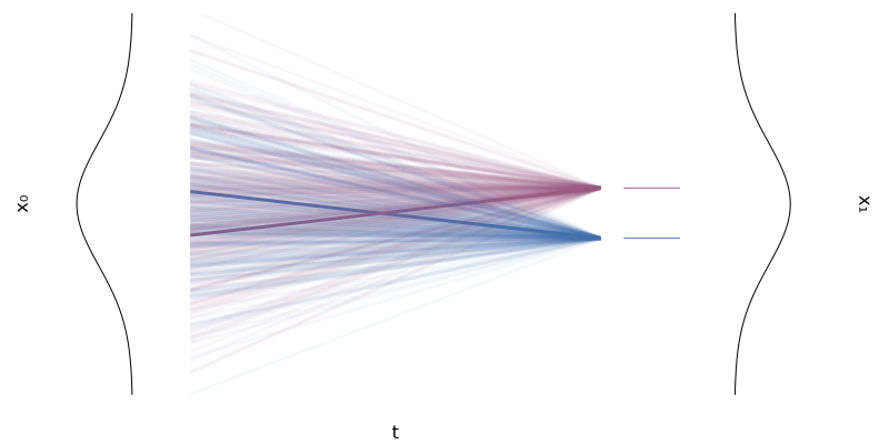
Inference

Step 1: Sample $x_0\sim\mathcal{N}(0,I_d)$
Step 2: Use a solver to solve the integral $x_1=x_0+\int_0^1 u_t(x_t)dt$

One note here is that we cannot predict the noise at level $0$ and subtract directly from $x_0$ in one step, but still we have to do this in multiple steps. The reason is quite simple. This is more or less like a linear approximation. The more you discretize the approximation, the more accurate it is. And the noise we predict will never be so accurate, but we can only approximate it to a certain level, so we "walk slowly in the right direction, and see where it brings us instead".

Duc Nguyen

Flow Matching